Genotype replacement in R

Estimate how fast a new dengue genotype takes over, with a logistic model fitted to sequence counts.

When a new genotype arrives, the share of sequences that belong to it often follows an S-shaped curve. A logistic model fitted to monthly sequence counts sums up the takeover in one number: how fast the odds of sampling the new genotype grow each month.

This tutorial uses simulated data, so you can check that the model recovers a known answer. You’ll need dplyr and ggplot2.

1. Simulate sequence counts

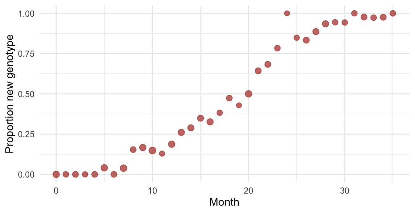
Three years of monthly sequencing, about 40 sequences a month, with the new genotype reaching half of all sequences in month 18.

library(dplyr)
library(ggplot2)

set.seed(42)

months <- 0:35
true_growth <- 0.25

seqs <- tibble(
  month = months,
  n = rpois(length(months), 40),
  new = rbinom(length(months), n, plogis(true_growth * (months - 18))),
  old = n - new
)

head(seqs)

# A tibble: 6 × 4
  month     n   new   old
  <int> <int> <int> <int>
1     0    48     0    48
2     1    36     0    36
3     2    40     0    40
4     3    33     0    33
5     4    39     0    39
6     5    49     2    47

2. Plot the raw proportions

ggplot(seqs, aes(month, new / n)) +
  geom_point(aes(size = n), colour = "#B2433A", alpha = 0.75) +
  scale_size_area(max_size = 3.5, guide = "none") +
  labs(x = "Month", y = "Proportion new genotype") +
  theme_minimal(base_size = 13)

Share of sequences belonging to the new genotype each month. Point size shows the number of sequences.

3. Fit a logistic model

A binomial GLM with month as the only predictor. The slope is the growth rate on the log-odds scale.

fit <- glm(cbind(new, old) ~ month, family = binomial, data = seqs)

coef(summary(fit))

              Estimate Std. Error   z value     Pr(>|z|)
(Intercept) -4.5876913 0.23203198 -19.77181 5.207782e-87
month        0.2516952 0.01222148  20.59449 3.075353e-94

4. Plot the fit

pred <- predict(fit, se.fit = TRUE)

seqs <- seqs |>
  mutate(
    fit = plogis(pred$fit),
    lo = plogis(pred$fit - 1.96 * pred$se.fit),
    hi = plogis(pred$fit + 1.96 * pred$se.fit)
  )

ggplot(seqs, aes(month)) +
  geom_ribbon(aes(ymin = lo, ymax = hi), fill = "#B2433A", alpha = 0.18) +
  geom_line(aes(y = fit), colour = "#B2433A", linewidth = 0.9) +
  geom_point(aes(y = new / n, size = n), colour = "#1D2930", alpha = 0.55) +
  scale_size_area(max_size = 3.5, guide = "none") +
  labs(x = "Month", y = "Proportion new genotype") +
  theme_minimal(base_size = 13)

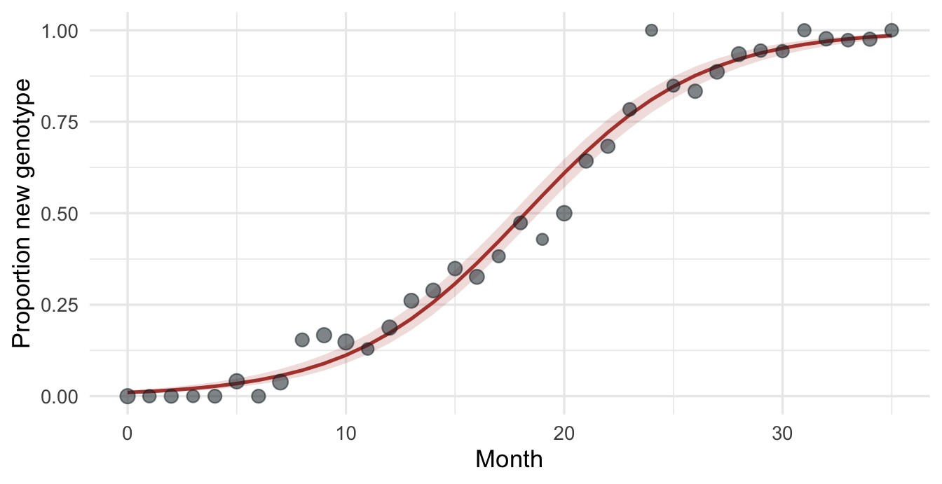
Fitted logistic curve with a 95% confidence interval.

5. Read off the growth advantage

growth <- coef(fit)[["month"]]

c(growth = growth, odds_ratio_per_month = exp(growth))

              growth odds_ratio_per_month 
           0.2516952            1.2862039 

The model estimates a growth rate of 0.25 per month against a true value of 0.25. Each month, the odds that a sequence belongs to the new genotype multiply by about 1.29.

NoteWith real data

Sequencing is rarely random. Check how samples were chosen for sequencing before reading the slope as a fitness advantage, and if you pool several places, consider a random effect for location.