Estimating Rt with a renewal equation

Methods

Tutorial

Simulate an outbreak from the renewal equation, then recover the time-varying reproduction number.

Published

October 22, 2026

The renewal equation says that new infections today depend on recent infections, weighted by the generation interval \(w_s\), the chance that \(s\) days separate an infection from the one it causes:

\[ I_t \sim \text{Poisson}\left(R_t \sum_{s \geq 1} I_{t-s}\, w_s\right) \]

This tutorial simulates an outbreak with a known \(R_t\), then estimates it back with the approach of Cori et al. (2013), written out in base R so every step is visible. You’ll need ggplot2 for the plots.

1. Set up the generation interval

A gamma distribution with a mean of six days, cut at three weeks.

library(ggplot2)

set.seed(1)

days <- 1:120
w <- dgamma(1:21, shape = 6, rate = 1)
w <- w / sum(w)

infectiousness <- function(inc, t) {
  s <- 1:min(t - 1, length(w))
  sum(inc[t - s] * w[s])
}

2. Simulate an outbreak

\(R_t\) is 1.5 until day 50, when a control measure brings it down to 0.8.

rt_true <- ifelse(days < 50, 1.5, 0.8)

inc <- numeric(length(days))
inc[1:5] <- 5

for (t in 6:length(days)) {
  inc[t] <- rpois(1, rt_true[t] * infectiousness(inc, t))
}

ggplot(data.frame(day = days, cases = inc), aes(day, cases)) +
  geom_col(fill = "#9A6714", width = 0.85) +
  labs(x = "Day", y = "Cases") +
  theme_minimal(base_size = 13)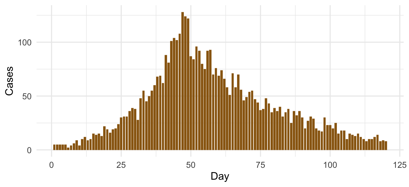

3. Estimate Rt over a sliding window

With a gamma prior on \(R_t\) (shape \(a\), scale \(b\)) and a window of \(\tau\) days, the posterior is also gamma, with shape \(a + \sum I_t\) and rate \(1/b + \sum \Lambda_t\), where \(\Lambda_t\) is the total infectiousness on day \(t\).

tau <- 7
a <- 1
b <- 5

lambda <- c(0, sapply(2:length(days), \(t) infectiousness(inc, t)))

est <- data.frame(day = 15:length(days))
est$shape <- sapply(est$day, \(t) a + sum(inc[(t - tau + 1):t]))
est$rate <- sapply(est$day, \(t) 1 / b + sum(lambda[(t - tau + 1):t]))
est$mean <- est$shape / est$rate
est$lo <- qgamma(0.025, est$shape, est$rate)
est$hi <- qgamma(0.975, est$shape, est$rate)

4. Compare with the truth

ggplot(est, aes(day)) +
  geom_hline(yintercept = 1, colour = "grey60", linewidth = 0.4) +
  geom_ribbon(aes(ymin = lo, ymax = hi), fill = "#9A6714", alpha = 0.25) +
  geom_line(aes(y = mean), colour = "#9A6714", linewidth = 0.9) +
  geom_step(data = data.frame(day = days, rt = rt_true), aes(y = rt), linetype = "dashed", colour = "#1D2930") +
  labs(x = "Day", y = expression(R[t])) +
  theme_minimal(base_size = 13)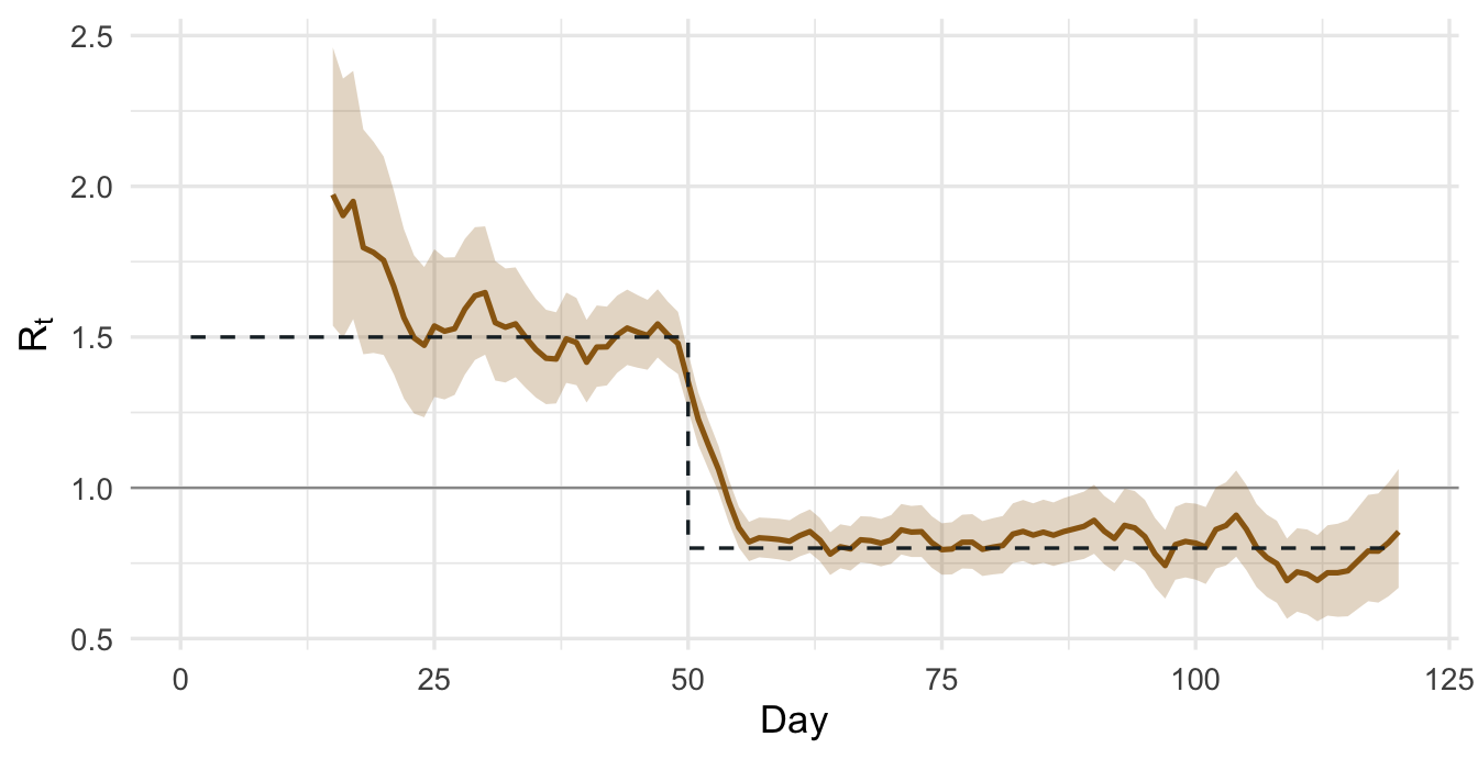

Estimated Rt with a 95% credible interval. The dashed line is the true value.

The estimate tracks the true \(R_t\) and takes about a window’s length to catch up after the drop on day 50.

For mosquito-borne viruses

The generation interval for dengue or chikungunya includes the time the virus spends developing inside the mosquito, so it is longer than for a respiratory virus and changes with temperature. Imported cases also need separating from local ones, or they inflate \(R_t\). See the chikungunya primer.